Logistic regression
Contents
Logistic regression#
In this chapter you will delve into the details of logistic regression. You’ll learn all about regularization and how to interpret model output.
Logistic regression and regularization#
Regularized logistic regression#
Regularized logistic regression
Hyperparameter C is the inverse of the regularization strength,
Larger C: less regularization,
Smaller C: more regularization,
Regularized loss = original loss + large coefficient penalty
More regularization: lower training accuracy,
More regularization: (almost always) higher test accuracy
L1 vs. L2 regularization
*Lasso = linear regression with L1 regularization, *Ridge = linear regression with L2 regularization,
In Chapter 1, you used logistic regression on the handwritten digits data set. Here, we’ll explore the effect of L2 regularization.
The handwritten digits dataset is already loaded, split, and stored in
the variables X_train, y_train,
X_valid, and y_valid. The variables
train_errs and valid_errs are already
initialized as empty lists.
C_value, creating and
fitting a LogisticRegression model each time.
C.
C?
# edited/added
from sklearn.datasets import load_digits

digits = load_digits()
X_train, X_valid, y_train, y_valid = train_test_split(digits.data, digits.target)
C_values = [0.001, 0.01, 0.1, 1, 10, 100, 1000]

# Train and validaton errors initialized as empty list
train_errs = list()
valid_errs = list()

# Loop over values of C_value
for C_value in [0.001, 0.01, 0.1, 1, 10, 100, 1000]:
    # Create LogisticRegression object and fit
    lr = LogisticRegression(C=C_value)
    lr.fit(X_train, y_train)

    # Evaluate error rates and append to lists
    train_errs.append( 1.0 - lr.score(X_train, y_train) )
    valid_errs.append( 1.0 - lr.score(X_valid, y_valid) )

# Plot results
## LogisticRegression(C=0.001)
## LogisticRegression(C=0.01)
## LogisticRegression(C=0.1)
## LogisticRegression(C=1)
## LogisticRegression(C=10)
## LogisticRegression(C=100)
## LogisticRegression(C=1000)
##
## /Users/macos/Library/r-miniconda/envs/r-reticulate/lib/python3.8/site-packages/sklearn/linear_model/_logistic.py:814: ConvergenceWarning: lbfgs failed to converge (status=1):
## STOP: TOTAL NO. of ITERATIONS REACHED LIMIT.
##
## Increase the number of iterations (max_iter) or scale the data as shown in:
## https://scikit-learn.org/stable/modules/preprocessing.html
## Please also refer to the documentation for alternative solver options:
## https://scikit-learn.org/stable/modules/linear_model.html#logistic-regression
## n_iter_i = _check_optimize_result(
plt.semilogx(C_values, train_errs, C_values, valid_errs)
plt.legend(("train", "validation"))
plt.show()
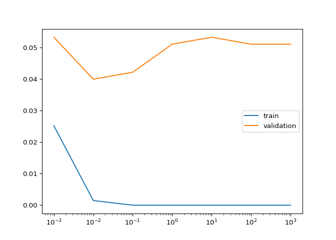
Congrats! As you can see, too much regularization (small C)
doesn’t work well - due to underfitting - and too little regularization
(large C) doesn’t work well either - due to overfitting.
Logistic regression and feature selection#
In this exercise we’ll perform feature selection on the movie review
sentiment data set using L1 regularization. The features and targets are
already loaded for you in X_train and y_train.
We’ll search for the best value of C using scikit-learn’s
GridSearchCV(), which was covered in the prerequisite
course.
C that minimizes cross-validation error.
C.
# edited/added
from sklearn.datasets import load_svmlight_file
from sklearn.model_selection import GridSearchCV

# edited/added
import numpy as np
from sklearn.datasets import load_svmlight_file
X_train, y_train = load_svmlight_file('archive/Linear-Classifiers-in-Python/datasets/train_labeledBow.feat')
X_train = X_train[11000:13000,:2500]
y_train = y_train[11000:13000]
y_train[y_train < 5] = -1.0
y_train[y_train >= 5] = 1.0

# Specify L1 regularization
lr = LogisticRegression(solver='liblinear', penalty='l1')

# Instantiate the GridSearchCV object and run the search
searcher = GridSearchCV(lr, {'C':[0.001, 0.01, 0.1, 1, 10]})
searcher.fit(X_train, y_train)

# Report the best parameters
## GridSearchCV(estimator=LogisticRegression(penalty='l1', solver='liblinear'),
##              param_grid={'C': [0.001, 0.01, 0.1, 1, 10]})
print("Best CV params", searcher.best_params_)

# Find the number of nonzero coefficients (selected features)
## Best CV params {'C': 0.1}
best_lr = searcher.best_estimator_
coefs = best_lr.coef_
print("Total number of features:", coefs.size)
## Total number of features: 2500
print("Number of selected features:", np.count_nonzero(coefs))
## Number of selected features: 143
Great job! As you can see, a whole lot of features were discarded here.
Identifying the most positive and negative words#
In this exercise we’ll try to interpret the coefficients of a logistic
regression fit on the movie review sentiment dataset. The model object
is already instantiated and fit for you in the variable lr.
In addition, the words corresponding to the different features are
loaded into the variable vocab. For example, since
vocab\[100\] is “think”, that means feature 100 corresponds
to the number of times the word “think” appeared in that movie review.
# edited/added
vocab = pd.read_csv('archive/Linear-Classifiers-in-Python/datasets/vocab.csv').to_numpy()

# Get the indices of the sorted cofficients
inds_ascending = np.argsort(best_lr.coef_.flatten())
inds_descending = inds_ascending[::-1]

# Print the most positive words
print("Most positive words: ", end="")
## Most positive words:
for i in range(5):
    print(vocab[inds_descending[i]], end=", ")
## ['great'], ['best'], ['our'], ['may'], ['enjoy'],
print("\n")

# Print most negative words
print("Most negative words: ", end="")
## Most negative words:
for i in range(5):
    print(vocab[inds_ascending[i]], end=", ")
## ['worst'], ['boring'], ['bad'], ['waste'], ['annoying'],
print("\n")
You got it! The answers sort of make sense, don’t they?
Logistic regression and probabilities#
Getting class probabilities#
Which of the following transformations would make sense for transforming the raw model output of a linear classifier into a class probability?

(1)
(2)
(3)
(4)
Regularization and probabilities#
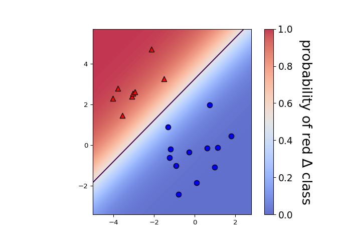
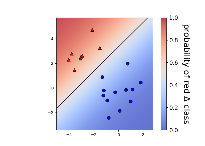
In this exercise, you will observe the effects of changing the regularization strength on the predicted probabilities.
A 2D binary classification dataset is already loaded into the
environment as X and y.
C=0.1 and examine how the plot and
probabilities change.
# edited/added
X = pd.read_csv('archive/Linear-Classifiers-in-Python/datasets/binary_X.csv').to_numpy()
y = pd.read_csv('archive/Linear-Classifiers-in-Python/datasets/binary_y.csv').to_numpy().ravel()

# Set the regularization strength
model = LogisticRegression(C=1)

# Fit and plot
model.fit(X,y)
## LogisticRegression(C=1)
plot_classifier(X,y,model,proba=True)

# Predict probabilities on training points
prob = model.predict_proba(X)
print("Maximum predicted probability", np.max(prob))

# Set the regularization strength
## Maximum predicted probability 0.9973143426900802
model = LogisticRegression(C=0.1)

# Fit and plot
model.fit(X,y)
## LogisticRegression(C=0.1)
plot_classifier(X,y,model,proba=True)

# Predict probabilities on training points
prob = model.predict_proba(X)
print("Maximum predicted probability", np.max(prob))
## Maximum predicted probability 0.9352061680350906
You got it! As you probably noticed, smaller values of C
lead to less confident predictions. That’s because smaller
C means more regularization, which in turn means smaller
coefficients, which means raw model outputs closer to zero and, thus,
probabilities closer to 0.5 after the raw model output is squashed
through the sigmoid function. That’s quite a chain of events!
Visualizing easy and difficult examples#
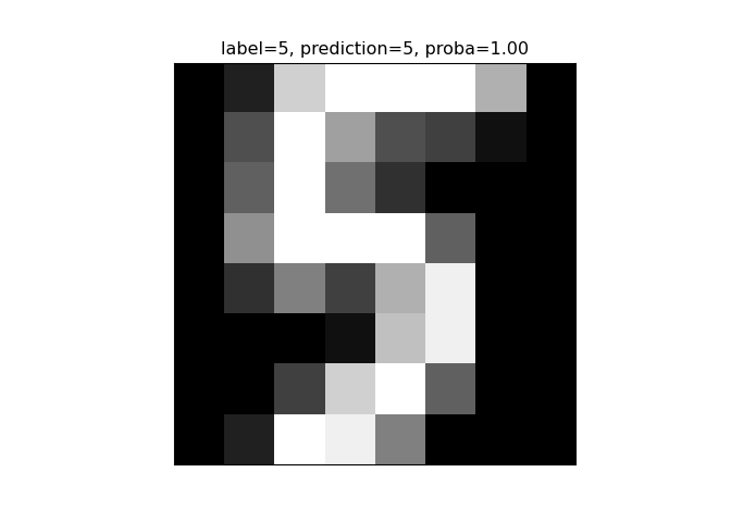
In this exercise, you’ll visualize the examples that the logistic regression model is most and least confident about by looking at the largest and smallest predicted probabilities.
The handwritten digits dataset is already loaded into the variables
X and y. The show_digit function
takes in an integer index and plots the corresponding image, with some
extra information displayed above the image.
# edited/added
def show_digit(i, lr=None):
    plt.imshow(np.reshape(X[i], (8,8)), cmap='gray',
               vmin = 0, vmax = 16, interpolation=None)
    plt.xticks(())
    plt.yticks(())
    if lr is None:
        plt.title("class label = %d" % y[i])
    else:
        pred = lr.predict(X[i][None])
        pred_prob = lr.predict_proba(X[i][None])[0,pred]
        plt.title("label=%d, prediction=%d, proba=%.2f" % (y[i], pred, pred_prob))
        plt.show()

X, y = digits.data, digits.target

lr = LogisticRegression()
lr.fit(X,y)

# Get predicted probabilities
## LogisticRegression()
##
## /Users/macos/Library/r-miniconda/envs/r-reticulate/lib/python3.8/site-packages/sklearn/linear_model/_logistic.py:814: ConvergenceWarning: lbfgs failed to converge (status=1):
## STOP: TOTAL NO. of ITERATIONS REACHED LIMIT.
##
## Increase the number of iterations (max_iter) or scale the data as shown in:
##     https://scikit-learn.org/stable/modules/preprocessing.html
## Please also refer to the documentation for alternative solver options:
##     https://scikit-learn.org/stable/modules/linear_model.html#logistic-regression
##   n_iter_i = _check_optimize_result(
proba = lr.predict_proba(X)

# Sort the example indices by their maximum probability
proba_inds = np.argsort(np.max(proba,axis=1))

# Show the most confident (least ambiguous) digit
show_digit(proba_inds[-1], lr)

# Show the least confident (most ambiguous) digit
show_digit(proba_inds[0], lr)
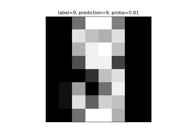
Great job! As you can see, the least confident example looks like a weird 9, and the most confident example looks like a very typical 5.
Multi-class logistic regression#
Counting the coefficients#
If you fit a logistic regression model on a classification problem with 3 classes and 100 features, how many coefficients would you have, including intercepts?
101
103
301
303
Fitting multi-class logistic regression#
In this exercise, you’ll fit the two types of multi-class logistic
regression, one-vs-rest and softmax/multinomial, on the handwritten
digits data set and compare the results. The handwritten digits dataset
is already loaded and split into X_train,
y_train, X_test, and y_test.
multi_class parameter and report the results.
multi_class parameter and report the results.
# edited/added
X_train, X_test, y_train, y_test = train_test_split(digits.data, digits.target)

# Fit one-vs-rest logistic regression classifier
lr_ovr = LogisticRegression(multi_class="ovr")
lr_ovr.fit(X_train, y_train)
## LogisticRegression(multi_class='ovr')
##
## /Users/macos/Library/r-miniconda/envs/r-reticulate/lib/python3.8/site-packages/sklearn/linear_model/_logistic.py:814: ConvergenceWarning: lbfgs failed to converge (status=1):
## STOP: TOTAL NO. of ITERATIONS REACHED LIMIT.
##
## Increase the number of iterations (max_iter) or scale the data as shown in:
## https://scikit-learn.org/stable/modules/preprocessing.html
## Please also refer to the documentation for alternative solver options:
## https://scikit-learn.org/stable/modules/linear_model.html#logistic-regression
## n_iter_i = _check_optimize_result(
print("OVR training accuracy:", lr_ovr.score(X_train, y_train))
## OVR training accuracy: 0.9985152190051967
print("OVR test accuracy    :", lr_ovr.score(X_test, y_test))

# Fit softmax classifier
## OVR test accuracy : 0.9622222222222222
lr_mn = LogisticRegression(multi_class="multinomial")
lr_mn.fit(X_train, y_train)
## LogisticRegression(multi_class='multinomial')
##
## /Users/macos/Library/r-miniconda/envs/r-reticulate/lib/python3.8/site-packages/sklearn/linear_model/_logistic.py:814: ConvergenceWarning: lbfgs failed to converge (status=1):
## STOP: TOTAL NO. of ITERATIONS REACHED LIMIT.
##
## Increase the number of iterations (max_iter) or scale the data as shown in:
##     https://scikit-learn.org/stable/modules/preprocessing.html
## Please also refer to the documentation for alternative solver options:
##     https://scikit-learn.org/stable/modules/linear_model.html#logistic-regression
##   n_iter_i = _check_optimize_result(
print("Softmax training accuracy:", lr_mn.score(X_train, y_train))
## Softmax training accuracy: 1.0
print("Softmax test accuracy :", lr_mn.score(X_test, y_test))
## Softmax test accuracy : 0.9622222222222222
Nice work! As you can see, the accuracies of the two methods are fairly similar on this data set.
Visualizing multi-class logistic regression#
In this exercise we’ll continue with the two types of multi-class logistic regression, but on a toy 2D data set specifically designed to break the one-vs-rest scheme.
The data set is loaded into X_train and
y_train. The two logistic regression
objects,lr_mn and lr_ovr, are already
instantiated (with C=100), fit, and plotted.
Notice that lr_ovr never predicts the dark blue class…
yikes! Let’s explore why this happens by plotting one of the binary
classifiers that it’s using behind the scenes.
C=100)
to be used for binary classification.
plot_classifier… does
it look reasonable?
# edited/added
X_train = pd.read_csv('archive/Linear-Classifiers-in-Python/datasets/toy_X_train.csv').to_numpy()
y_train = pd.read_csv('archive/Linear-Classifiers-in-Python/datasets/toy_y_train.csv').to_numpy().ravel()

lr_ovr = LogisticRegression(max_iter=10000, C=100)
lr_ovr.fit(X_train, y_train)
## LogisticRegression(C=100, max_iter=10000)
fig, ax = plt.subplots();
ax.set_title("lr_ovr (one-vs-rest)");
plot_classifier(X_train, y_train, lr_ovr, ax=ax);

lr_mn = LogisticRegression(multi_class='multinomial', solver='lbfgs', max_iter=10000)
lr_mn.fit(X_train, y_train)
## LogisticRegression(max_iter=10000, multi_class='multinomial')
fig, ax = plt.subplots();
ax.set_title("lr_mn (softmax)");
plot_classifier(X_train, y_train, lr_ovr, ax=ax);

# Print training accuracies
print("Softmax training accuracy:", lr_mn.score(X_train, y_train))
## Softmax training accuracy: 0.952
print("One-vs-rest training accuracy:", lr_ovr.score(X_train, y_train))

# Create the binary classifier (class 1 vs. rest)
## One-vs-rest training accuracy: 0.996
lr_class_1 = LogisticRegression(C=100)
lr_class_1.fit(X_train, y_train==1)

# Plot the binary classifier (class 1 vs. rest)
## LogisticRegression(C=100)
plot_classifier(X_train, y_train==1, lr_class_1)
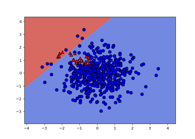
Nice work! As you can see, the binary classifier incorrectly labels almost all points in class 1 (shown as red triangles in the final plot)! Thus, this classifier is not a very effective component of the one-vs-rest classifier. In general, though, one-vs-rest often works well.
One-vs-rest SVM#
As motivation for the next and final chapter on support vector machines,
we’ll repeat the previous exercise with a non-linear SVM. Once again,
the data is loaded into X_train, y_train,
X_test, and y_test .
Instead of using LinearSVC, we’ll now use scikit-learn’s
SVC object, which is a non-linear “kernel” SVM (much more
on what this means in Chapter 4!). Again, your task is to create a plot
of the binary classifier for class 1 vs. rest.
SVC called svm_class_1 to predict class
1 vs. other classes.
# edited/added
X_test = pd.read_csv('archive/Linear-Classifiers-in-Python/datasets/toy_X_test.csv').to_numpy()
y_test = pd.read_csv('archive/Linear-Classifiers-in-Python/datasets/toy_y_test.csv').to_numpy().ravel()

# We'll use SVC instead of LinearSVC from now on
from sklearn.svm import SVC

# Create/plot the binary classifier (class 1 vs. rest)
svm_class_1 = SVC()
svm_class_1.fit(X_train, y_train==1)
## SVC()
plot_classifier(X_train, y_train==1, svm_class_1)
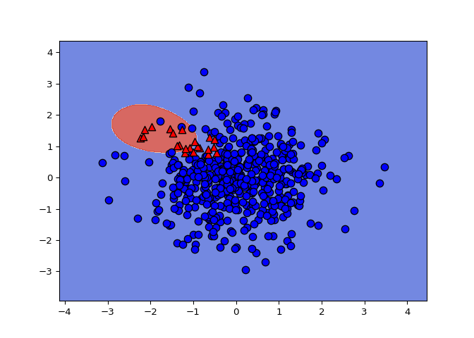
Cool, eh?! The non-linear SVM works fine with one-vs-rest on this dataset because it learns to “surround” class 1.
