Support Vector Machines
Contents
Support Vector Machines#
In this chapter you will learn all about the details of support vector machines. You’ll learn about tuning hyperparameters for these models and using kernels to fit non-linear decision boundaries.
Support vectors#
Support vector definition#
Which of the following is a true statement about support vectors? To help you out, here’s the picture of support vectors from the video (top), as well as the hinge loss from Chapter 2 (bottom).


All support vectors are classified correctly.
All support vectors are classified incorrectly.
All correctly classified points are support vectors.
All incorrectly classified points are support vectors.
Effect of removing examples#
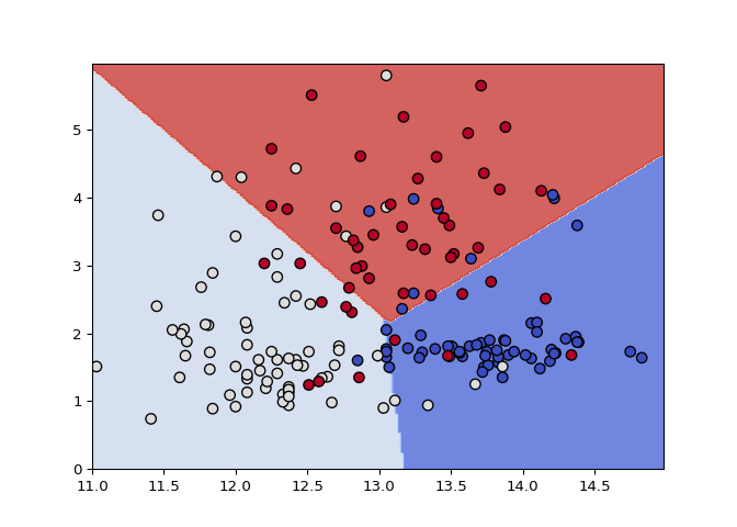
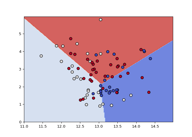
Support vectors are defined as training examples that influence the decision boundary. In this exercise, you’ll observe this behavior by removing non support vectors from the training set.
The wine quality dataset is already loaded into X and
y (first two features only). (Note: we specify
lims in plot_classifier() so that the two
plots are forced to use the same axis limits and can be compared
directly.)
# edited/added
X = pd.read_csv('archive/Linear-Classifiers-in-Python/datasets/wine_X.csv').to_numpy()
y = pd.read_csv('archive/Linear-Classifiers-in-Python/datasets/wine_y.csv').to_numpy().ravel()

# Train a linear SVM
svm = SVC(kernel="linear")
svm.fit(X,y)
## SVC(kernel='linear')
plot_classifier(X, y, svm, lims=(11,15,0,6))

# Make a new data set keeping only the support vectors

print("Number of original examples", len(X))
## Number of original examples 178
print("Number of support vectors", len(svm.support_))
## Number of support vectors 81
X_small = X[svm.support_]
y_small = y[svm.support_]

# Train a new SVM using only the support vectors
svm_small = SVC(kernel="linear")
svm_small.fit(X_small, y_small)
## SVC(kernel='linear')
plot_classifier(X_small, y_small, svm_small, lims=(11,15,0,6))

Nice! Compare the decision boundaries of the two trained models: are they the same? By the definition of support vectors, they should be!
Kernel SVMs#
GridSearchCV warm-up#
In the video we saw that increasing the RBF kernel hyperparameter
gamma increases training accuracy. In this exercise we’ll
search for the gamma that maximizes cross-validation
accuracy using scikit-learn’s GridSearchCV. A binary
version of the handwritten digits dataset, in which you’re just trying
to predict whether or not an image is a “2”, is already loaded into the
variables X and y.
GridSearchCV object.
fit() method to select the best value of
gamma based on cross-validation accuracy.
# edited/added
X = pd.read_csv('archive/Linear-Classifiers-in-Python/datasets/digits_2_X.csv').to_numpy()
y = pd.read_csv('archive/Linear-Classifiers-in-Python/datasets/digits_2_y.csv').astype('bool').to_numpy().ravel()

# Instantiate an RBF SVM
svm = SVC()

# Instantiate the GridSearchCV object and run the search
parameters = {'gamma':[0.00001, 0.0001, 0.001, 0.01, 0.1]}
searcher = GridSearchCV(svm, parameters)
searcher.fit(X, y)

# Report the best parameters
## GridSearchCV(estimator=SVC(),
##              param_grid={'gamma': [1e-05, 0.0001, 0.001, 0.01, 0.1]})
print("Best CV params", searcher.best_params_)
## Best CV params {'gamma': 0.001}
Great job! Larger values of gamma are better for training
accuracy, but cross-validation helped us find something different (and
better!).
Jointly tuning gamma and C with GridSearchCV#
In the previous exercise the best value of gamma was 0.001
using the default value of C, which is 1. In this exercise
you’ll search for the best combination of C and
gamma using GridSearchCV.
As in the previous exercise, the 2-vs-not-2 digits dataset is already
loaded, but this time it’s split into the variables
X_train, y_train, X_test, and
y_test. Even though cross-validation already splits the
training set into parts, it’s often a good idea to hold out a separate
test set to make sure the cross-validation results are sensible.
GridSearchCV to find the best hyperparameters using the
training set.
# edited/added
from sklearn.model_selection import train_test_split
X_train, X_test, y_train, y_test = train_test_split(X, y)

# Instantiate an RBF SVM
svm = SVC()

# Instantiate the GridSearchCV object and run the search
parameters = {'C':[0.1, 1, 10], 'gamma':[0.00001, 0.0001, 0.001, 0.01, 0.1]}
searcher = GridSearchCV(svm, parameters)
searcher.fit(X_train, y_train)

# Report the best parameters and the corresponding score
## GridSearchCV(estimator=SVC(),
##              param_grid={'C': [0.1, 1, 10],
##                          'gamma': [1e-05, 0.0001, 0.001, 0.01, 0.1]})
print("Best CV params", searcher.best_params_)
## Best CV params {'C': 1, 'gamma': 0.001}
print("Best CV accuracy", searcher.best_score_)

# Report the test accuracy using these best parameters
## Best CV accuracy 0.9970259812050857
print("Test accuracy of best grid search hypers:", searcher.score(X_test, y_test))
## Test accuracy of best grid search hypers: 1.0
You got it! Note that the best value of gamma, 0.0001, is
different from the value of 0.001 that we got in the previous exercise,
when we fixed C=1. Hyperparameters can affect each other!
Comparing logistic regression and SVM#
Logistic regression:
Is a linear classifier
Can use with kernels, but slow
Outputs meaningful probabilities
Can be extended to multi-class
All data points affect fit
L2 or L1 regularization
Support Vector Machine (SVM)
Is a linear classifier
Can use with kernels, and fast
Does not naturally output probabilities
Can be extended to multi-class
Only “support vectors” affect fit
Conventionally just L2 regularization
An advantage of SVMs#
Which of the following is an advantage of SVMs over logistic regression?
They naturally output meaningful probabilities.
They can be used with kernels.
They are computationally efficient with kernels.
They learn sigmoidal decision boundaries.
An advantage of logistic regression#
Which of the following is an advantage of logistic regression over SVMs?
It naturally outputs meaningful probabilities.
It can be used with kernels.
It is computationally efficient with kernels.
It learns sigmoidal decision boundaries.
Using SGDClassifier#
In this final coding exercise, you’ll do a hyperparameter search over
the regularization strength and the loss (logistic regression vs. linear
SVM) using SGDClassifier().
SGDClassifier instance with
random_state=0.
hinge
vs. log_loss losses.
# edited/added
from sklearn.linear_model import SGDClassifier
X, y = digits.data, digits.target
X_train, X_test, y_train, y_test = train_test_split(X, y)

# We set random_state=0 for reproducibility
linear_classifier = SGDClassifier(random_state=0)

# Instantiate the GridSearchCV object and run the search
parameters = {'alpha':[0.00001, 0.0001, 0.001, 0.01, 0.1, 1],
             'loss':['hinge', 'log_loss']}
searcher = GridSearchCV(linear_classifier, parameters, cv=10)
searcher.fit(X_train, y_train)

# Report the best parameters and the corresponding score
## GridSearchCV(cv=10, estimator=SGDClassifier(random_state=0),
##              param_grid={'alpha': [1e-05, 0.0001, 0.001, 0.01, 0.1, 1],
##                          'loss': ['hinge', 'log_loss']})
##
## /Users/macos/Library/r-miniconda/envs/r-reticulate/lib/python3.8/site-packages/sklearn/model_selection/_validation.py:372: FitFailedWarning:
## 60 fits failed out of a total of 120.
## The score on these train-test partitions for these parameters will be set to nan.
## If these failures are not expected, you can try to debug them by setting error_score='raise'.
##
## Below are more details about the failures:
## --------------------------------------------------------------------------------
## 60 fits failed with the following error:
## Traceback (most recent call last):
##   File "/Users/macos/Library/r-miniconda/envs/r-reticulate/lib/python3.8/site-packages/sklearn/model_selection/_validation.py", line 681, in _fit_and_score
##     estimator.fit(X_train, y_train, **fit_params)
##   File "/Users/macos/Library/r-miniconda/envs/r-reticulate/lib/python3.8/site-packages/sklearn/linear_model/_stochastic_gradient.py", line 890, in fit
##     return self._fit(
##   File "/Users/macos/Library/r-miniconda/envs/r-reticulate/lib/python3.8/site-packages/sklearn/linear_model/_stochastic_gradient.py", line 649, in _fit
##     self._validate_params()
##   File "/Users/macos/Library/r-miniconda/envs/r-reticulate/lib/python3.8/site-packages/sklearn/linear_model/_stochastic_gradient.py", line 162, in _validate_params
##     raise ValueError("The loss %s is not supported. " % self.loss)
## ValueError: The loss log_loss is not supported.
##
##   warnings.warn(some_fits_failed_message, FitFailedWarning)
## /Users/macos/Library/r-miniconda/envs/r-reticulate/lib/python3.8/site-packages/sklearn/model_selection/_search.py:969: UserWarning: One or more of the test scores are non-finite: [0.93391376        nan 0.94656716        nan 0.94062465        nan
##  0.94730238        nan 0.95101161        nan 0.95252626        nan]
##   warnings.warn(
print("Best CV params", searcher.best_params_)
## Best CV params {'alpha': 1, 'loss': 'hinge'}
print("Best CV accuracy", searcher.best_score_)
## Best CV accuracy 0.9525262576008844
print("Test accuracy of best grid search hypers:", searcher.score(X_test, y_test))
## Test accuracy of best grid search hypers: 0.9511111111111111
Congrats, you finished the last exercise in the course! One advantage of
SGDClassifier is that it’s very fast - this would have
taken a lot longer with LogisticRegression or
LinearSVC.
Conclusion#
Conclusion#
You made it - congratulations!
How does this course fit into data science?#
You now have practice applying logistic regression and support vector machines to classification problems. How does this fit into a bigger picture? The way I see it, data science is the process of answering questions and making decisions based on data. The data science process usually combines several of the following pieces: data collection, data preparation, database design, visualization, communication, software engineering, machine learning, and more. In this course we focused on the machine learning portion. Machine learning has several branches like supervised learning, unsupervised learning, and reinforcement learning. We’ve been focusing on supervised learning, which means trying to predict a target value from features given a labeled data set. Within supervised learning, we’ve focussed on classification, which means the thing we’re trying to predict is categorical rather than a continuous in nature. Finally, we covered logistic regression and SVMs, the two most popular linear classifiers. So, while we’ve done a lot, there’s so much more out there!
Congratulations & thanks!#
Thanks for completing this journey with me. I hope you enjoyed it as much as I did. Congratulations again.
