Visualization with hierarchical clustering and t-SNE#

In this chapter, you’ll learn about two unsupervised learning techniques for data visualization, hierarchical clustering and t-SNE. Hierarchical clustering merges the data samples into ever-coarser clusters, yielding a tree visualization of the resulting cluster hierarchy. t-SNE maps the data samples into 2d space so that the proximity of the samples to one another can be visualized.

Visualizing hierarchies#

How many merges?#

If there are 5 data samples, how many merge operations will occur in a hierarchical clustering? (To help answer this question, think back to the video, in which Ben walked through an example of hierarchical clustering using 6 countries.)

4 merges.
3 merges.
This can’t be known in advance.

Well done! With 5 data samples, there would be 4 merge operations, and with 6 data samples, there would be 5 merges, and so on.

Hierarchical clustering of the grain data#

In the video, you learned that the SciPy linkage() function performs hierarchical clustering on an array of samples. Use the linkage() function to obtain a hierarchical clustering of the grain samples, and use dendrogram() to visualize the result. A sample of the grain measurements is provided in the array samples, while the variety of each grain sample is given by the list varieties.

Import:

linkage and dendrogram from scipy.cluster.hierarchy.

matplotlib.pyplot as plt.

Perform hierarchical clustering on samples using the linkage() function with the method=‘complete’ keyword argument. Assign the result to mergings.

Plot a dendrogram using the dendrogram() function on mergings. Specify the keyword arguments labels=varieties, leaf_rotation=90, and leaf_font_size=6.

# edited/added
samples = np.array(grains.sample(42))[:,:7]
varieties = list(np.array(grains.sample(42))[:,8])

# Perform the necessary imports
from scipy.cluster.hierarchy import linkage, dendrogram
import matplotlib.pyplot as plt

# Calculate the linkage: mergings
mergings = linkage(samples, method='complete')

# Plot the dendrogram, using varieties as labels
dendrogram(mergings,
           labels=varieties,
           leaf_rotation=90,
           leaf_font_size=6,
)

## {'icoord': [[25.0, 25.0, 35.0, 35.0], [15.0, 15.0, 30.0, 30.0], [55.0, 55.0, 65.0, 65.0], [45.0, 45.0, 60.0, 60.0], [22.5, 22.5, 52.5, 52.5], [5.0, 5.0, 37.5, 37.5], [85.0, 85.0, 95.0, 95.0], [105.0, 105.0, 115.0, 115.0], [125.0, 125.0, 135.0, 135.0], [110.0, 110.0, 130.0, 130.0], [145.0, 145.0, 155.0, 155.0], [165.0, 165.0, 175.0, 175.0], [150.0, 150.0, 170.0, 170.0], [120.0, 120.0, 160.0, 160.0], [90.0, 90.0, 140.0, 140.0], [75.0, 75.0, 115.0, 115.0], [185.0, 185.0, 195.0, 195.0], [205.0, 205.0, 215.0, 215.0], [225.0, 225.0, 235.0, 235.0], [255.0, 255.0, 265.0, 265.0], [245.0, 245.0, 260.0, 260.0], [230.0, 230.0, 252.5, 252.5], [210.0, 210.0, 241.25, 241.25], [190.0, 190.0, 225.625, 225.625], [275.0, 275.0, 285.0, 285.0], [305.0, 305.0, 315.0, 315.0], [295.0, 295.0, 310.0, 310.0], [280.0, 280.0, 302.5, 302.5], [207.8125, 207.8125, 291.25, 291.25], [345.0, 345.0, 355.0, 355.0], [335.0, 335.0, 350.0, 350.0], [325.0, 325.0, 342.5, 342.5], [375.0, 375.0, 385.0, 385.0], [405.0, 405.0, 415.0, 415.0], [395.0, 395.0, 410.0, 410.0], [380.0, 380.0, 402.5, 402.5], [365.0, 365.0, 391.25, 391.25], [333.75, 333.75, 378.125, 378.125], [249.53125, 249.53125, 355.9375, 355.9375], [95.0, 95.0, 302.734375, 302.734375], [21.25, 21.25, 198.8671875, 198.8671875]], 'dcoord': [[0.0, 0.35892177420713867, 0.35892177420713867, 0.0], [0.0, 0.6444799531405162, 0.6444799531405162, 0.35892177420713867], [0.0, 0.6327327160816018, 0.6327327160816018, 0.0], [0.0, 1.57472866234155, 1.57472866234155, 0.6327327160816018], [0.6444799531405162, 2.1906390300549288, 2.1906390300549288, 1.57472866234155], [0.0, 3.8753454671809577, 3.8753454671809577, 2.1906390300549288], [0.0, 0.7207984184222385, 0.7207984184222385, 0.0], [0.0, 0.3449266008877837, 0.3449266008877837, 0.0], [0.0, 0.5373874300725677, 0.5373874300725677, 0.0], [0.3449266008877837, 1.0132117251591595, 1.0132117251591595, 0.5373874300725677], [0.0, 0.4019535296523724, 0.4019535296523724, 0.0], [0.0, 0.74000216891574, 0.74000216891574, 0.0], [0.4019535296523724, 1.1923667892054022, 1.1923667892054022, 0.74000216891574], [1.0132117251591595, 1.7057229229860276, 1.7057229229860276, 1.1923667892054022], [0.7207984184222385, 2.76135637142329, 2.76135637142329, 1.7057229229860276], [0.0, 4.8292916664869185, 4.8292916664869185, 2.76135637142329], [0.0, 0.8213969137998998, 0.8213969137998998, 0.0], [0.0, 0.7680247456950849, 0.7680247456950849, 0.0], [0.0, 0.39210953826705036, 0.39210953826705036, 0.0], [0.0, 0.44020218082149526, 0.44020218082149526, 0.0], [0.0, 0.6878648122996261, 0.6878648122996261, 0.44020218082149526], [0.39210953826705036, 0.8667876095099653, 0.8667876095099653, 0.6878648122996261], [0.7680247456950849, 1.6315417279371072, 1.6315417279371072, 0.8667876095099653], [0.8213969137998998, 2.0021865947009037, 2.0021865947009037, 1.6315417279371072], [0.0, 0.7600501365041651, 0.7600501365041651, 0.0], [0.0, 0.4355730593138186, 0.4355730593138186, 0.0], [0.0, 0.8899149172814218, 0.8899149172814218, 0.4355730593138186], [0.7600501365041651, 2.2825246898993226, 2.2825246898993226, 0.8899149172814218], [2.0021865947009037, 3.108696229933058, 3.108696229933058, 2.2825246898993226], [0.0, 0.28514601522728705, 0.28514601522728705, 0.0], [0.0, 1.0559243533511296, 1.0559243533511296, 0.28514601522728705], [0.0, 2.196101828240212, 2.196101828240212, 1.0559243533511296], [0.0, 0.5513404120867617, 0.5513404120867617, 0.0], [0.0, 0.5540343761897811, 0.5540343761897811, 0.0], [0.0, 0.8413507235392381, 0.8413507235392381, 0.5540343761897811], [0.5513404120867617, 1.6519585981494824, 1.6519585981494824, 0.8413507235392381], [0.0, 2.6224088640027143, 2.6224088640027143, 1.6519585981494824], [2.196101828240212, 4.713556156449182, 4.713556156449182, 2.6224088640027143], [3.108696229933058, 5.923029677453931, 5.923029677453931, 4.713556156449182], [4.8292916664869185, 8.159839861173747, 8.159839861173747, 5.923029677453931], [3.8753454671809577, 10.666543593873321, 10.666543593873321, 8.159839861173747]], 'ivl': ['Kama wheat', 'Kama wheat', 'Rosa wheat', 'Kama wheat', 'Rosa wheat', 'Rosa wheat', 'Rosa wheat', 'Kama wheat', 'Canadian wheat', 'Canadian wheat', 'Canadian wheat', 'Rosa wheat', 'Canadian wheat', 'Rosa wheat', 'Rosa wheat', 'Kama wheat', 'Canadian wheat', 'Rosa wheat', 'Kama wheat', 'Canadian wheat', 'Kama wheat', 'Canadian wheat', 'Rosa wheat', 'Canadian wheat', 'Canadian wheat', 'Rosa wheat', 'Canadian wheat', 'Rosa wheat', 'Rosa wheat', 'Rosa wheat', 'Canadian wheat', 'Kama wheat', 'Kama wheat', 'Canadian wheat', 'Kama wheat', 'Rosa wheat', 'Rosa wheat', 'Canadian wheat', 'Rosa wheat', 'Rosa wheat', 'Kama wheat', 'Canadian wheat'], 'leaves': [32, 8, 6, 16, 39, 1, 34, 10, 9, 29, 14, 26, 5, 18, 3, 22, 7, 11, 13, 21, 15, 31, 28, 38, 20, 19, 30, 0, 33, 4, 2, 41, 40, 17, 27, 37, 36, 24, 35, 25, 12, 23], 'color_list': ['C1', 'C1', 'C1', 'C1', 'C1', 'C1', 'C2', 'C2', 'C2', 'C2', 'C2', 'C2', 'C2', 'C2', 'C2', 'C2', 'C3', 'C3', 'C3', 'C3', 'C3', 'C3', 'C3', 'C3', 'C3', 'C3', 'C3', 'C3', 'C3', 'C3', 'C3', 'C3', 'C3', 'C3', 'C3', 'C3', 'C3', 'C3', 'C3', 'C0', 'C0']}

plt.show()

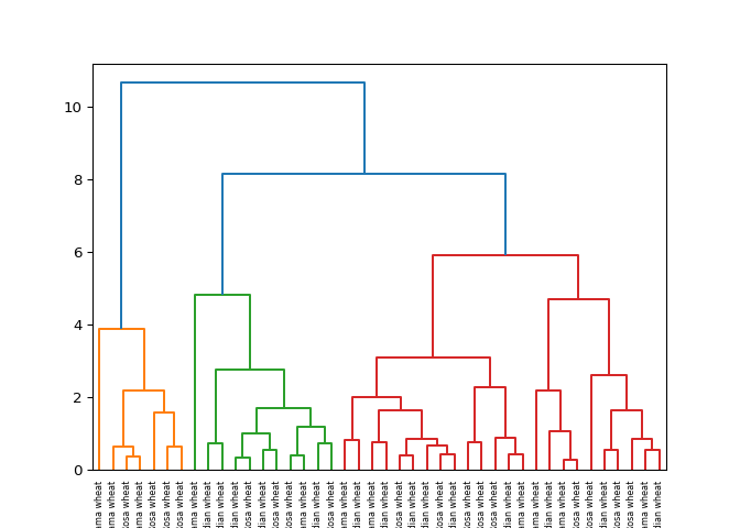
Superb! Dendrograms are a great way to illustrate the arrangement of the clusters produced by hierarchical clustering.

Hierarchies of stocks#

In chapter 1, you used k-means clustering to cluster companies according to their stock price movements. Now, you’ll perform hierarchical clustering of the companies. You are given a NumPy array of price movements movements, where the rows correspond to companies, and a list of the company names companies. SciPy hierarchical clustering doesn’t fit into a sklearn pipeline, so you’ll need to use the normalize() function from sklearn.preprocessing instead of Normalizer.

linkage and dendrogram have already been imported from scipy.cluster.hierarchy, and PyPlot has been imported as plt.

Import normalize from sklearn.preprocessing.

Rescale the price movements for each stock by using the normalize() function on movements.

Apply the linkage() function to normalized_movements, using ‘complete’ linkage, to calculate the hierarchical clustering. Assign the result to mergings.

Plot a dendrogram of the hierarchical clustering, using the list companies of company names as the labels. In addition, specify the leaf_rotation=90, and leaf_font_size=6 keyword arguments as you did in the previous exercise.

# Import normalize
from sklearn.preprocessing import normalize

# Normalize the movements: normalized_movements
normalized_movements = normalize(movements)

# Calculate the linkage: mergings
mergings = linkage(normalized_movements, method='complete')

# Plot the dendrogram
dendrogram(
    mergings,
    labels=companies,
    leaf_rotation=90,
    leaf_font_size=6
)

## {'icoord': [[25.0, 25.0, 35.0, 35.0], [15.0, 15.0, 30.0, 30.0], [45.0, 45.0, 55.0, 55.0], [75.0, 75.0, 85.0, 85.0], [65.0, 65.0, 80.0, 80.0], [50.0, 50.0, 72.5, 72.5], [22.5, 22.5, 61.25, 61.25], [5.0, 5.0, 41.875, 41.875], [105.0, 105.0, 115.0, 115.0], [95.0, 95.0, 110.0, 110.0], [175.0, 175.0, 185.0, 185.0], [165.0, 165.0, 180.0, 180.0], [155.0, 155.0, 172.5, 172.5], [145.0, 145.0, 163.75, 163.75], [205.0, 205.0, 215.0, 215.0], [235.0, 235.0, 245.0, 245.0], [225.0, 225.0, 240.0, 240.0], [210.0, 210.0, 232.5, 232.5], [195.0, 195.0, 221.25, 221.25], [154.375, 154.375, 208.125, 208.125], [295.0, 295.0, 305.0, 305.0], [285.0, 285.0, 300.0, 300.0], [275.0, 275.0, 292.5, 292.5], [265.0, 265.0, 283.75, 283.75], [345.0, 345.0, 355.0, 355.0], [335.0, 335.0, 350.0, 350.0], [325.0, 325.0, 342.5, 342.5], [315.0, 315.0, 333.75, 333.75], [274.375, 274.375, 324.375, 324.375], [255.0, 255.0, 299.375, 299.375], [181.25, 181.25, 277.1875, 277.1875], [135.0, 135.0, 229.21875, 229.21875], [125.0, 125.0, 182.109375, 182.109375], [102.5, 102.5, 153.5546875, 153.5546875], [23.4375, 23.4375, 128.02734375, 128.02734375], [365.0, 365.0, 375.0, 375.0], [395.0, 395.0, 405.0, 405.0], [425.0, 425.0, 435.0, 435.0], [415.0, 415.0, 430.0, 430.0], [400.0, 400.0, 422.5, 422.5], [385.0, 385.0, 411.25, 411.25], [370.0, 370.0, 398.125, 398.125], [465.0, 465.0, 475.0, 475.0], [455.0, 455.0, 470.0, 470.0], [445.0, 445.0, 462.5, 462.5], [485.0, 485.0, 495.0, 495.0], [535.0, 535.0, 545.0, 545.0], [525.0, 525.0, 540.0, 540.0], [515.0, 515.0, 532.5, 532.5], [505.0, 505.0, 523.75, 523.75], [565.0, 565.0, 575.0, 575.0], [555.0, 555.0, 570.0, 570.0], [514.375, 514.375, 562.5, 562.5], [490.0, 490.0, 538.4375, 538.4375], [585.0, 585.0, 595.0, 595.0], [514.21875, 514.21875, 590.0, 590.0], [453.75, 453.75, 552.109375, 552.109375], [384.0625, 384.0625, 502.9296875, 502.9296875], [75.732421875, 75.732421875, 443.49609375, 443.49609375]], 'dcoord': [[0.0, 0.8766150964619032, 0.8766150964619032, 0.0], [0.0, 1.0052496265150068, 1.0052496265150068, 0.8766150964619032], [0.0, 1.0405854841254667, 1.0405854841254667, 0.0], [0.0, 0.9756642737984944, 0.9756642737984944, 0.0], [0.0, 1.0443532462900014, 1.0443532462900014, 0.9756642737984944], [1.0405854841254667, 1.1087706867538036, 1.1087706867538036, 1.0443532462900014], [1.0052496265150068, 1.1539599583553475, 1.1539599583553475, 1.1087706867538036], [0.0, 1.1953921911777048, 1.1953921911777048, 1.1539599583553475], [0.0, 1.0675113301764332, 1.0675113301764332, 0.0], [0.0, 1.162102133265849, 1.162102133265849, 1.0675113301764332], [0.0, 0.6937115853632807, 0.6937115853632807, 0.0], [0.0, 0.7897669950447856, 0.7897669950447856, 0.6937115853632807], [0.0, 0.9060804298422901, 0.9060804298422901, 0.7897669950447856], [0.0, 0.9978691096150067, 0.9978691096150067, 0.9060804298422901], [0.0, 0.850608403749446, 0.850608403749446, 0.0], [0.0, 0.7506255354591677, 0.7506255354591677, 0.0], [0.0, 0.8894957237528659, 0.8894957237528659, 0.7506255354591677], [0.850608403749446, 0.9615815807943434, 0.9615815807943434, 0.8894957237528659], [0.0, 1.0334597062675297, 1.0334597062675297, 0.9615815807943434], [0.9978691096150067, 1.05365593648412, 1.05365593648412, 1.0334597062675297], [0.0, 0.8528392636699416, 0.8528392636699416, 0.0], [0.0, 0.8730000088242031, 0.8730000088242031, 0.8528392636699416], [0.0, 0.9595547992508179, 0.9595547992508179, 0.8730000088242031], [0.0, 0.9933139902556245, 0.9933139902556245, 0.9595547992508179], [0.0, 0.6735509755390415, 0.6735509755390415, 0.0], [0.0, 0.7984090019882444, 0.7984090019882444, 0.6735509755390415], [0.0, 0.8794722330700889, 0.8794722330700889, 0.7984090019882444], [0.0, 1.0410874279228417, 1.0410874279228417, 0.8794722330700889], [0.9933139902556245, 1.0581735997075004, 1.0581735997075004, 1.0410874279228417], [0.0, 1.115596724887607, 1.115596724887607, 1.0581735997075004], [1.05365593648412, 1.1659596038210138, 1.1659596038210138, 1.115596724887607], [0.0, 1.1700635570314206, 1.1700635570314206, 1.1659596038210138], [0.0, 1.1909309430336361, 1.1909309430336361, 1.1700635570314206], [1.162102133265849, 1.236510636000957, 1.236510636000957, 1.1909309430336361], [1.1953921911777048, 1.2467384602108724, 1.2467384602108724, 1.236510636000957], [0.0, 1.1224902285374243, 1.1224902285374243, 0.0], [0.0, 0.9516416111189119, 0.9516416111189119, 0.0], [0.0, 0.9263737672939854, 0.9263737672939854, 0.0], [0.0, 0.9774020092313027, 0.9774020092313027, 0.9263737672939854], [0.9516416111189119, 1.0825651898927742, 1.0825651898927742, 0.9774020092313027], [0.0, 1.1436387132254562, 1.1436387132254562, 1.0825651898927742], [1.1224902285374243, 1.1617351684882877, 1.1617351684882877, 1.1436387132254562], [0.0, 0.804091365214309, 0.804091365214309, 0.0], [0.0, 0.9529466260111008, 0.9529466260111008, 0.804091365214309], [0.0, 1.1381811890921898, 1.1381811890921898, 0.9529466260111008], [0.0, 1.0014106416309905, 1.0014106416309905, 0.0], [0.0, 0.58499795491215, 0.58499795491215, 0.0], [0.0, 0.78536856335178, 0.78536856335178, 0.58499795491215], [0.0, 0.8427599656210099, 0.8427599656210099, 0.78536856335178], [0.0, 0.88159190249364, 0.88159190249364, 0.8427599656210099], [0.0, 0.8547176535466976, 0.8547176535466976, 0.0], [0.0, 0.917129270573618, 0.917129270573618, 0.8547176535466976], [0.88159190249364, 1.0113079675726626, 1.0113079675726626, 0.917129270573618], [1.0014106416309905, 1.0903568915580981, 1.0903568915580981, 1.0113079675726626], [0.0, 1.1116148749505466, 1.1116148749505466, 0.0], [1.0903568915580981, 1.1665446301937066, 1.1665446301937066, 1.1116148749505466], [1.1381811890921898, 1.203388148166268, 1.203388148166268, 1.1665446301937066], [1.1617351684882877, 1.2625272906988811, 1.2625272906988811, 1.203388148166268], [1.2467384602108724, 1.3161900463070635, 1.3161900463070635, 1.2625272906988811]], 'ivl': ['Apple', 'Taiwan Semiconductor Manufacturing', 'Intel', 'Texas instruments', 'Dell', 'HP', 'Symantec', 'Cisco', 'Microsoft', 'Yahoo', 'Amazon', 'Google/Alphabet', 'AIG', 'Valero Energy', 'American express', 'Goldman Sachs', 'Wells Fargo', 'Bank of America', 'JPMorgan Chase', 'Ford', 'Canon', 'Sony', 'Mitsubishi', 'Honda', 'Toyota', 'Navistar', 'IBM', 'General Electrics', '3M', 'Caterpillar', 'DuPont de Nemours', 'Xerox', 'Schlumberger', 'ConocoPhillips', 'Chevron', 'Exxon', 'Home Depot', 'Wal-Mart', 'Philip Morris', 'Coca Cola', 'Pepsi', 'Kimberly-Clark', 'Colgate-Palmolive', 'Procter Gamble', 'Walgreen', 'Boeing', 'Lookheed Martin', 'Northrop Grumman', 'Johnson & Johnson', 'Pfizer', 'SAP', 'Sanofi-Aventis', 'Unilever', 'Royal Dutch Shell', 'Total', 'British American Tobacco', 'GlaxoSmithKline', 'Novartis', 'MasterCard', 'McDonalds'], 'leaves': [0, 50, 24, 51, 14, 22, 47, 11, 33, 59, 2, 17, 1, 53, 3, 18, 55, 5, 26, 15, 7, 45, 34, 21, 48, 35, 23, 16, 32, 8, 13, 58, 44, 10, 12, 57, 20, 56, 41, 28, 38, 27, 9, 40, 54, 4, 29, 36, 25, 39, 43, 46, 52, 42, 49, 6, 19, 37, 30, 31], 'color_list': ['C1', 'C0', 'C0', 'C0', 'C0', 'C0', 'C0', 'C0', 'C0', 'C0', 'C2', 'C2', 'C2', 'C0', 'C3', 'C4', 'C4', 'C0', 'C0', 'C0', 'C5', 'C5', 'C0', 'C0', 'C6', 'C6', 'C6', 'C0', 'C0', 'C0', 'C0', 'C0', 'C0', 'C0', 'C0', 'C0', 'C0', 'C0', 'C0', 'C0', 'C0', 'C0', 'C7', 'C0', 'C0', 'C0', 'C8', 'C8', 'C8', 'C8', 'C9', 'C9', 'C0', 'C0', 'C0', 'C0', 'C0', 'C0', 'C0']}

plt.show()

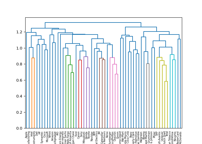
Great work! You can produce great visualizations such as this with hierarchical clustering, but it can be used for more than just visualizations. You’ll find out more about this in the next video!

Cluster labels in hierarchical clustering#

Which clusters are closest?#

In the video, you learned that the linkage method defines how the distance between clusters is measured. In complete linkage, the distance between clusters is the distance between the furthest points of the clusters. In single linkage, the distance between clusters is the distance between the closest points of the clusters.

Consider the three clusters in the diagram. Which of the following statements are true?

A. In single linkage, Cluster 3 is the closest cluster to Cluster 2.

B. In complete linkage, Cluster 1 is the closest cluster to Cluster 2.

Neither A nor B.
A only.
Both A and B.

Well done!

Different linkage, different hierarchical clustering!#

In the video, you saw a hierarchical clustering of the voting countries at the Eurovision song contest using ‘complete’ linkage. Now, perform a hierarchical clustering of the voting countries with ‘single’ linkage, and compare the resulting dendrogram with the one in the video. Different linkage, different hierarchical clustering!

You are given an array samples. Each row corresponds to a voting country, and each column corresponds to a performance that was voted for. The list country_names gives the name of each voting country. This dataset was obtained from Eurovision.

Import linkage and dendrogram from scipy.cluster.hierarchy.

Perform hierarchical clustering on samples using the linkage() function with the method=‘single’ keyword argument. Assign the result to mergings.

Plot a dendrogram of the hierarchical clustering, using the list country_names as the labels. In addition, specify the leaf_rotation=90, and leaf_font_size=6 keyword arguments as you have done earlier.

# edited/added
eurovision = pd.read_csv("archive/Unsupervised-Learning-in-Python/datasets/eurovision-2016.csv").fillna(0)
scores = pd.crosstab(index=eurovision['From country'], columns=eurovision['To country'], values=eurovision['Televote Points'], aggfunc='first').fillna(12)
samples = scores.values
country_names = list(scores.index)

# Perform the necessary imports
import matplotlib.pyplot as plt
from scipy.cluster.hierarchy import linkage, dendrogram

# Calculate the linkage: mergings
mergings = linkage(samples, method='single')

# Plot the dendrogram
dendrogram(mergings,
           labels=country_names,
           leaf_rotation=90,
           leaf_font_size=6,
)

## {'icoord': [[15.0, 15.0, 25.0, 25.0], [65.0, 65.0, 75.0, 75.0], [85.0, 85.0, 95.0, 95.0], [70.0, 70.0, 90.0, 90.0], [105.0, 105.0, 115.0, 115.0], [80.0, 80.0, 110.0, 110.0], [55.0, 55.0, 95.0, 95.0], [135.0, 135.0, 145.0, 145.0], [185.0, 185.0, 195.0, 195.0], [175.0, 175.0, 190.0, 190.0], [265.0, 265.0, 275.0, 275.0], [255.0, 255.0, 270.0, 270.0], [245.0, 245.0, 262.5, 262.5], [235.0, 235.0, 253.75, 253.75], [315.0, 315.0, 325.0, 325.0], [355.0, 355.0, 365.0, 365.0], [345.0, 345.0, 360.0, 360.0], [335.0, 335.0, 352.5, 352.5], [320.0, 320.0, 343.75, 343.75], [375.0, 375.0, 385.0, 385.0], [405.0, 405.0, 415.0, 415.0], [395.0, 395.0, 410.0, 410.0], [380.0, 380.0, 402.5, 402.5], [331.875, 331.875, 391.25, 391.25], [305.0, 305.0, 361.5625, 361.5625], [295.0, 295.0, 333.28125, 333.28125], [285.0, 285.0, 314.140625, 314.140625], [244.375, 244.375, 299.5703125, 299.5703125], [225.0, 225.0, 271.97265625, 271.97265625], [215.0, 215.0, 248.486328125, 248.486328125], [205.0, 205.0, 231.7431640625, 231.7431640625], [182.5, 182.5, 218.37158203125, 218.37158203125], [165.0, 165.0, 200.435791015625, 200.435791015625], [155.0, 155.0, 182.7178955078125, 182.7178955078125], [140.0, 140.0, 168.85894775390625, 168.85894775390625], [125.0, 125.0, 154.42947387695312, 154.42947387695312], [75.0, 75.0, 139.71473693847656, 139.71473693847656], [45.0, 45.0, 107.35736846923828, 107.35736846923828], [35.0, 35.0, 76.17868423461914, 76.17868423461914], [20.0, 20.0, 55.58934211730957, 55.58934211730957], [5.0, 5.0, 37.794671058654785, 37.794671058654785]], 'dcoord': [[0.0, 9.273618495495704, 9.273618495495704, 0.0], [0.0, 7.211102550927978, 7.211102550927978, 0.0], [0.0, 10.488088481701515, 10.488088481701515, 0.0], [7.211102550927978, 12.0, 12.0, 10.488088481701515], [0.0, 13.114877048604, 13.114877048604, 0.0], [12.0, 13.564659966250536, 13.564659966250536, 13.114877048604], [0.0, 15.874507866387544, 15.874507866387544, 13.564659966250536], [0.0, 14.7648230602334, 14.7648230602334, 0.0], [0.0, 6.782329983125268, 6.782329983125268, 0.0], [0.0, 11.045361017187261, 11.045361017187261, 6.782329983125268], [0.0, 8.94427190999916, 8.94427190999916, 0.0], [0.0, 11.224972160321824, 11.224972160321824, 8.94427190999916], [0.0, 12.083045973594572, 12.083045973594572, 11.224972160321824], [0.0, 12.083045973594572, 12.083045973594572, 12.083045973594572], [0.0, 8.0, 8.0, 0.0], [0.0, 8.366600265340756, 8.366600265340756, 0.0], [0.0, 9.797958971132712, 9.797958971132712, 8.366600265340756], [0.0, 9.899494936611665, 9.899494936611665, 9.797958971132712], [8.0, 10.862780491200215, 10.862780491200215, 9.899494936611665], [0.0, 9.38083151964686, 9.38083151964686, 0.0], [0.0, 10.583005244258363, 10.583005244258363, 0.0], [0.0, 11.224972160321824, 11.224972160321824, 10.583005244258363], [9.38083151964686, 11.224972160321824, 11.224972160321824, 11.224972160321824], [10.862780491200215, 11.313708498984761, 11.313708498984761, 11.224972160321824], [0.0, 11.40175425099138, 11.40175425099138, 11.313708498984761], [0.0, 11.661903789690601, 11.661903789690601, 11.40175425099138], [0.0, 13.416407864998739, 13.416407864998739, 11.661903789690601], [12.083045973594572, 13.711309200802088, 13.711309200802088, 13.416407864998739], [0.0, 14.071247279470288, 14.071247279470288, 13.711309200802088], [0.0, 14.142135623730951, 14.142135623730951, 14.071247279470288], [0.0, 14.142135623730951, 14.142135623730951, 14.142135623730951], [11.045361017187261, 14.491376746189438, 14.491376746189438, 14.142135623730951], [0.0, 14.628738838327793, 14.628738838327793, 14.491376746189438], [0.0, 15.937377450509228, 15.937377450509228, 14.628738838327793], [14.7648230602334, 16.55294535724685, 16.55294535724685, 15.937377450509228], [0.0, 16.911534525287763, 16.911534525287763, 16.55294535724685], [15.874507866387544, 17.204650534085253, 17.204650534085253, 16.911534525287763], [0.0, 17.663521732655695, 17.663521732655695, 17.204650534085253], [0.0, 17.72004514666935, 17.72004514666935, 17.663521732655695], [9.273618495495704, 18.384776310850235, 18.384776310850235, 17.72004514666935], [0.0, 19.79898987322333, 19.79898987322333, 18.384776310850235]], 'ivl': ['Australia', 'Belgium', 'The Netherlands', 'Spain', 'Italy', 'Switzerland', 'Croatia', 'Slovenia', 'Bosnia & Herzegovina', 'Montenegro', 'F.Y.R. Macedonia', 'Serbia', 'Malta', 'France', 'Israel', 'Albania', 'Azerbaijan', 'Bulgaria', 'Cyprus', 'Greece', 'Czech Republic', 'Armenia', 'Germany', 'Russia', 'Moldova', 'Georgia', 'Belarus', 'Ukraine', 'Austria', 'Hungary', 'United Kingdom', 'Ireland', 'Norway', 'Estonia', 'San Marino', 'Latvia', 'Lithuania', 'Denmark', 'Iceland', 'Sweden', 'Finland', 'Poland'], 'leaves': [2, 6, 39, 36, 24, 38, 9, 35, 7, 29, 14, 34, 27, 16, 23, 0, 4, 8, 10, 19, 11, 1, 18, 32, 28, 17, 5, 40, 3, 20, 41, 22, 30, 13, 33, 25, 26, 12, 21, 37, 15, 31], 'color_list': ['C1', 'C2', 'C2', 'C2', 'C2', 'C2', 'C0', 'C0', 'C3', 'C3', 'C4', 'C4', 'C4', 'C4', 'C4', 'C4', 'C4', 'C4', 'C4', 'C4', 'C4', 'C4', 'C4', 'C4', 'C4', 'C4', 'C4', 'C4', 'C0', 'C0', 'C0', 'C0', 'C0', 'C0', 'C0', 'C0', 'C0', 'C0', 'C0', 'C0', 'C0']}

plt.show()

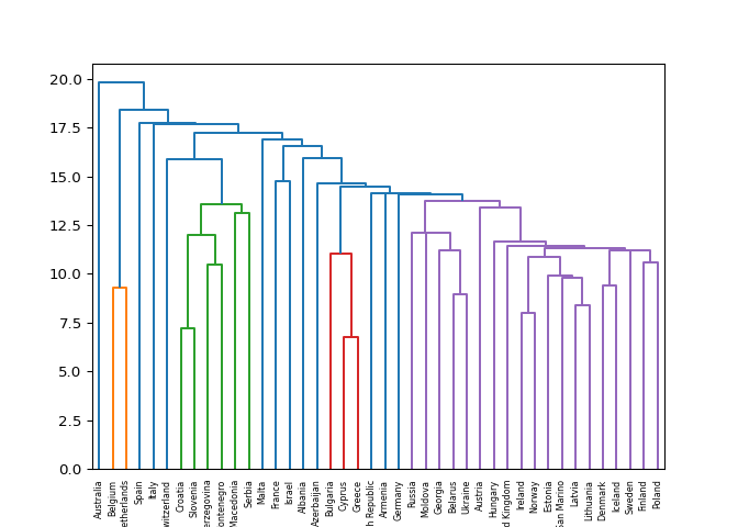
Great work! As you can see, performing single linkage hierarchical clustering produces a different dendrogram!

Intermediate clusterings#

Displayed on the right is the dendrogram for the hierarchical clustering of the grain samples that you computed earlier. If the hierarchical clustering were stopped at height 6 on the dendrogram, how many clusters would there be?

1.
3.
As many as there were at the beginning.

Exactly - great work!

Extracting the cluster labels#

In the previous exercise, you saw that the intermediate clustering of the grain samples at height 6 has 3 clusters. Now, use the fcluster() function to extract the cluster labels for this intermediate clustering, and compare the labels with the grain varieties using a cross-tabulation.

The hierarchical clustering has already been performed and mergings is the result of the linkage() function. The list varieties gives the variety of each grain sample.

Import:

pandas as pd.

fcluster from scipy.cluster.hierarchy.

Perform a flat hierarchical clustering by using the fcluster() function on mergings. Specify a maximum height of 6 and the keyword argument criterion=‘distance’.

Create a DataFrame df with two columns named ‘labels’ and ‘varieties’, using labels and varieties, respectively, for the column values. This has been done for you.

Create a cross-tabulation ct between df\[‘labels’\] and df\[‘varieties’\] to count the number of times each grain variety coincides with each cluster label.

# edited/added
samples = np.array(grains.sample(42))[:,:7]
varieties = list(np.array(grains.sample(42))[:,8])
mergings = linkage(samples, method='complete')

# Perform the necessary imports
import pandas as pd
from scipy.cluster.hierarchy import fcluster

# Use fcluster to extract labels: labels
labels = fcluster(mergings, 6, criterion='distance')

# Create a DataFrame with labels and varieties as columns: df
df = pd.DataFrame({'labels': labels, 'varieties': varieties})

# Create crosstab: ct
ct = pd.crosstab(df['labels'], df['varieties'])

# Display ct
print(ct)

## varieties  Canadian wheat  Kama wheat  Rosa wheat
## labels                                           
## 1                       1           4           2
## 2                       4           6           2
## 3                       6           9           8

Fantastic - you’ve now mastered the fundamentals of k-Means and agglomerative hierarchical clustering. Next, you’ll learn about t-SNE, which is a powerful tool for visualizing high dimensional data.

t-SNE for 2-dimensional maps#

t-SNE visualization of grain dataset#

In the video, you saw t-SNE applied to the iris dataset. In this exercise, you’ll apply t-SNE to the grain samples data and inspect the resulting t-SNE features using a scatter plot. You are given an array samples of grain samples and a list variety_numbers giving the variety number of each grain sample.

Import TSNE from sklearn.manifold.

Create a TSNE instance called model with learning_rate=200.

Apply the .fit_transform() method of model to samples. Assign the result to tsne_features.

Select the column 0 of tsne_features. Assign the result to xs.

Select the column 1 of tsne_features. Assign the result to ys.

Make a scatter plot of the t-SNE features xs and ys. To color the points by the grain variety, specify the additional keyword argument c=variety_numbers.

# edited/added
variety_numbers = list(np.array(grains.sample(42))[:,7])

# Import TSNE
from sklearn.manifold import TSNE

# Create a TSNE instance: model
model = TSNE(learning_rate=200)

# Apply fit_transform to samples: tsne_features
tsne_features = model.fit_transform(samples)

# Select the 0th feature: xs
xs = tsne_features[:,0]

# Select the 1st feature: ys
ys = tsne_features[:,1]

# Scatter plot, coloring by variety_numbers
plt.scatter(xs, ys, c=variety_numbers)
plt.show()

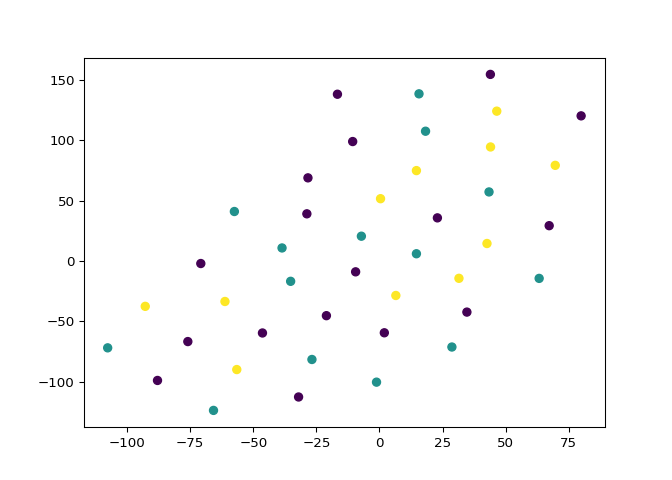
Excellent! As you can see, the t-SNE visualization manages to separate the 3 varieties of grain samples. But how will it perform on the stock data? You’ll find out in the next exercise!

A t-SNE map of the stock market#

t-SNE provides great visualizations when the individual samples can be labeled. In this exercise, you’ll apply t-SNE to the company stock price data. A scatter plot of the resulting t-SNE features, labeled by the company names, gives you a map of the stock market! The stock price movements for each company are available as the array normalized_movements (these have already been normalized for you). The list companies gives the name of each company. PyPlot (plt) has been imported for you.

Import TSNE from sklearn.manifold.

Create a TSNE instance called model with learning_rate=50.

Apply the .fit_transform() method of model to normalized_movements. Assign the result to tsne_features.

Select column 0 and column 1 of tsne_features.

Make a scatter plot of the t-SNE features xs and ys. Specify the additional keyword argument alpha=0.5.

Code to label each point with its company name has been written for you using plt.annotate(), so just hit submit to see the visualization!

# edited/added
import numpy as np
import pandas as pd
import matplotlib.pyplot as plt
from sklearn.preprocessing import normalize
stock = np.array(pd.read_csv("archive/Unsupervised-Learning-in-Python/datasets/company-stock-movements-2010-2015-incl.csv", header = None, skiprows=1))
movements = stock[:,1:]
companies = list(stock[:,0])
normalized_movements = normalize(movements)

# Import TSNE
from sklearn.manifold import TSNE

# Create a TSNE instance: model
model = TSNE(learning_rate=50)

# Apply fit_transform to normalized_movements: tsne_features
tsne_features = model.fit_transform(normalized_movements)

# Select the 0th feature: xs
xs = tsne_features[:,0]

# Select the 1th feature: ys
ys = tsne_features[:,1]

# Scatter plot
plt.scatter(xs, ys, alpha=0.5)

# Annotate the points
for x, y, company in zip(xs, ys, companies):
    plt.annotate(company, (x, y), fontsize=5, alpha=0.75)
plt.show()

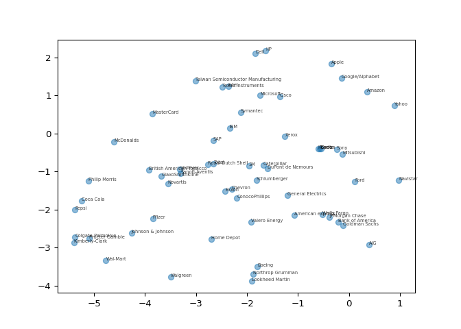
Fantastic! It’s visualizations such as this that make t-SNE such a powerful tool for extracting quick insights from high dimensional data.

Machine Learning Scientist with Python

Visualization with hierarchical clustering and t-SNE

Contents