Decorrelating your data and dimension reduction
Contents
Decorrelating your data and dimension reduction#
Dimension reduction summarizes a dataset using its common occuring patterns. In this chapter, you’ll learn about the most fundamental of dimension reduction techniques, “Principal Component Analysis” (“PCA”). PCA is often used before supervised learning to improve model performance and generalization. It can also be useful for unsupervised learning. For example, you’ll employ a variant of PCA will allow you to cluster Wikipedia articles by their content!
Visualizing the PCA transformation#
Decorrelating the grain measurements with PCA#
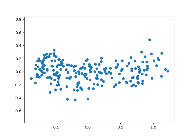
You observed in the previous exercise that the width and length measurements of the grain are correlated. Now, you’ll use PCA to decorrelate these measurements, then plot the decorrelated points and measure their Pearson correlation.
PCA from sklearn.decomposition.
PCA called model.
.fit_transform() method of model to
apply the PCA transformation to grains. Assign the result
to pca_features.
pca_features has been
written for you, so hit submit to see the result!
# Import PCA
from sklearn.decomposition import PCA
# Create PCA instance: model
model = PCA()
# Apply the fit_transform method of model to grains: pca_features
pca_features = model.fit_transform(grains)
# Assign 0th column of pca_features: xs
xs = pca_features[:,0]
# Assign 1st column of pca_features: ys
ys = pca_features[:,1]
# Scatter plot xs vs ys
plt.scatter(xs, ys)
plt.axis('equal')
## (-0.9666954859113024, 1.3255192221382366, -0.47614840965670485, 0.5348749465462598)
plt.show()

# Calculate the Pearson correlation of xs and ys

correlation, pvalue = pearsonr(xs, ys)

# Display the correlation
print(correlation)
## 8.933825901280557e-17
Excellent! You’ve successfully decorrelated the grain measurements with PCA!
Principal components#
On the right are three scatter plots of the same point cloud. Each scatter plot shows a different set of axes (in red). In which of the plots could the axes represent the principal components of the point cloud?
Recall that the principal components are the directions along which the the data varies.

None of them.
Both plot 1 and plot 3.
Plot 2.
Well done! You’ve correctly inferred that the principal components have to align with the axes of the point cloud. This happens in both plot 1 and plot 3.
Intrinsic dimension#
The first principal component#
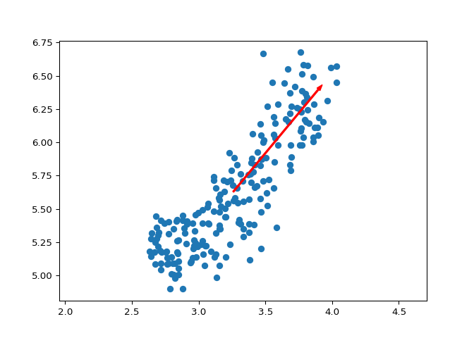
The first principal component of the data is the direction in which the data varies the most. In this exercise, your job is to use PCA to find the first principal component of the length and width measurements of the grain samples, and represent it as an arrow on the scatter plot.
The array grains gives the length and width of the grain
samples. PyPlot (plt) and PCA have already
been imported for you.
PCA instance called model.
grains data.
.mean\_ attribute of model.
model using the
.components\_\[0,:\] attribute.
plt.arrow() function. You have to specify the
first two arguments - mean\[0\] and mean\[1\].
# Make a scatter plot of the untransformed points
plt.scatter(grains[:,0], grains[:,1])

# Create a PCA instance: model
model = PCA()

# Fit model to points
model.fit(grains)

# Get the mean of the grain samples: mean
## PCA()
mean = model.mean_

# Get the first principal component: first_pc
first_pc = model.components_[0,:]

# Plot first_pc as an arrow, starting at mean
plt.arrow(mean[0], mean[1], first_pc[0], first_pc[1], color='red', width=0.01)

# Keep axes on same scale
plt.axis('equal')
## (2.55985, 4.10315, 4.8102, 6.7638)
plt.show()

Excellent job! This is the direction in which the grain data varies the most.
Variance of the PCA features#
The fish dataset is 6-dimensional. But what is its intrinsic
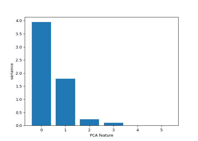
dimension? Make a plot of the variances of the PCA features to find out.
As before, samples is a 2D array, where each row represents
a fish. You’ll need to standardize the features first.
StandardScaler called
scaler.
PCA instance called pca.
make_pipeline() function to create a pipeline
chaining scaler and pca.
.fit() method of pipeline to fit it to
the fish samples samples.
.n_components\_ attribute of pca. Place this
inside a range() function and store the result as
features.
plt.bar() function to plot the explained variances,
with features on the x-axis and
pca.explained_variance\_ on the y-axis.
# edited/added
fish = np.array(pd.read_csv("archive/Unsupervised-Learning-in-Python/datasets/fish.csv", header = None))
samples = fish[:,1:]
species = fish[:,0]

# Perform the necessary imports
from sklearn.decomposition import PCA
from sklearn.preprocessing import StandardScaler
from sklearn.pipeline import make_pipeline
import matplotlib.pyplot as plt

# Create scaler: scaler
scaler = StandardScaler()

# Create a PCA instance: pca
pca = PCA()

# Create pipeline: pipeline
pipeline = make_pipeline(scaler, pca)

# Fit the pipeline to 'samples'
pipeline.fit(samples)

# Plot the explained variances
## Pipeline(steps=[('standardscaler', StandardScaler()), ('pca', PCA())])
features = range(pca.n_components_)

plt.bar(features, pca.explained_variance_)
## <BarContainer object of 6 artists>
plt.xlabel('PCA feature')
plt.ylabel('variance')
plt.xticks(features)
## ([<matplotlib.axis.XTick object at 0x7ffcd9269cd0>, <matplotlib.axis.XTick object at 0x7ffcd9269f40>, <matplotlib.axis.XTick object at 0x7ffcd5657850>, <matplotlib.axis.XTick object at 0x7ffcd922e610>, <matplotlib.axis.XTick object at 0x7ffcd92137c0>, <matplotlib.axis.XTick object at 0x7ffcdacd1c70>], [Text(0, 0, ''), Text(0, 0, ''), Text(0, 0, ''), Text(0, 0, ''), Text(0, 0, ''), Text(0, 0, '')])
plt.show()

Great work! It looks like PCA features 0 and 1 have significant variance.
Intrinsic dimension of the fish data#
In the previous exercise, you plotted the variance of the PCA features of the fish measurements. Looking again at your plot, what do you think would be a reasonable choice for the “intrinsic dimension” of the fish measurements? Recall that the intrinsic dimension is the number of PCA features with significant variance.
1
2
5
Great job! Since PCA features 0 and 1 have significant variance, the intrinsic dimension of this dataset appears to be 2.
Dimension reduction with PCA#
Dimension reduction#
In a previous exercise, you saw that 2 was a reasonable
choice for the “intrinsic dimension” of the fish measurements. Now use
PCA for dimensionality reduction of the fish measurements, retaining
only the 2 most important components.
The fish measurements have already been scaled for you, and are
available as scaled_samples.
PCA from sklearn.decomposition.
pca with
n_components=2.
.fit() method of pca to fit it to the
scaled fish measurements scaled_samples.
.transform() method of pca to
transform the scaled_samples. Assign the result to
pca_features.
# edited/added
scaler = StandardScaler()
scaled_samples = scaler.fit_transform(samples)

# Import PCA
from sklearn.decomposition import PCA

# Create a PCA instance with 2 components: pca
pca = PCA(n_components=2)

# Fit the PCA instance to the scaled samples
pca.fit(scaled_samples)

# Transform the scaled samples: pca_features
## PCA(n_components=2)
pca_features = pca.transform(scaled_samples)

# Print the shape of pca_features
print(pca_features.shape)
## (85, 2)
Superb! You’ve successfully reduced the dimensionality from 6 to 2.
A tf-idf word-frequency array#
In this exercise, you’ll create a tf-idf word frequency array for a toy
collection of documents. For this, use the TfidfVectorizer
from sklearn. It transforms a list of documents into a word frequency
array, which it outputs as a csr_matrix. It has fit() and
transform() methods like other sklearn objects.
You are given a list documents of toy documents about pets.
Its contents have been printed in the IPython Shell.
TfidfVectorizer from
sklearn.feature_extraction.text.
TfidfVectorizer instance called
tfidf.
.fit_transform() method of tfidf to
documents and assign the result to csr_mat.
This is a word-frequency array in csr_matrix format.
csr_mat by calling its .toarray()
method and printing the result. This has been done for you.
.get_feature_names() method of
tfidf, and assign the result to words.
# edited/added
documents = ['cats say meow', 'dogs say woof', 'dogs chase cats']

# Import TfidfVectorizer
from sklearn.feature_extraction.text import TfidfVectorizer

# Create a TfidfVectorizer: tfidf
tfidf = TfidfVectorizer()

# Apply fit_transform to document: csr_mat
csr_mat = tfidf.fit_transform(documents)

# Print result of toarray() method
print(csr_mat.toarray())

# Get the words: words
## [[0.51785612 0.         0.         0.68091856 0.51785612 0.        ]
##  [0.         0.         0.51785612 0.         0.51785612 0.68091856]
##  [0.51785612 0.68091856 0.51785612 0.         0.         0.        ]]
words = tfidf.get_feature_names()

# Print words
print(words)
## ['cats', 'chase', 'dogs', 'meow', 'say', 'woof']
Great work! You’ll now move to clustering Wikipedia articles!
Clustering Wikipedia part I#
You saw in the video that TruncatedSVD is able to perform
PCA on sparse arrays in csr_matrix format, such as word-frequency
arrays. Combine your knowledge of TruncatedSVD and k-means to cluster
some popular pages from Wikipedia. In this exercise, build the pipeline.
In the next exercise, you’ll apply it to the word-frequency array of
some Wikipedia articles.
Create a Pipeline object consisting of a TruncatedSVD followed by KMeans. (This time, we’ve precomputed the word-frequency matrix for you, so there’s no need for a TfidfVectorizer).
The Wikipedia dataset you will be working with was obtained from here.
TruncatedSVD from sklearn.decomposition.
KMeans from sklearn.cluster.
make_pipeline from sklearn.pipeline.
TruncatedSVD instance called svd with
n_components=50.
KMeans instance called kmeans with
n_clusters=6.
pipeline consisting of
svd and kmeans.
# Perform the necessary imports
from sklearn.decomposition import TruncatedSVD
from sklearn.cluster import KMeans
from sklearn.pipeline import make_pipeline

# Create a TruncatedSVD instance: svd
svd = TruncatedSVD(n_components=50)

# Create a KMeans instance: kmeans
kmeans = KMeans(n_clusters=6)

# Create a pipeline: pipeline
pipeline = make_pipeline(svd, kmeans)
Excellent! Now that you have set up your pipeline, you will use it in the next exercise to cluster the articles.
Clustering Wikipedia part II#
It is now time to put your pipeline from the previous exercise to work!
You are given an array articles of tf-idf word-frequencies
of some popular Wikipedia articles, and a list titles of
their titles. Use your pipeline to cluster the Wikipedia articles.
A solution to the previous exercise has been pre-loaded for you, so a
Pipeline pipeline chaining TruncatedSVD with KMeans is
available.
pandas as pd.
articles.
titles of article
titles by creating a DataFrame df with labels
and titles as columns. This has been done for you.
.sort_values() method of df to sort
the DataFrame by the ‘label’ column, and print the result.
# edited/added
from scipy.sparse import csc_matrix
documents = pd.read_csv('archive/Unsupervised-Learning-in-Python/datasets/wikipedia-vectors.csv', index_col=0)
titles = documents.columns
articles = csc_matrix(documents.values).T

# Import pandas
import pandas as pd

# Fit the pipeline to articles
pipeline.fit(articles)

# Calculate the cluster labels: labels
## Pipeline(steps=[('truncatedsvd', TruncatedSVD(n_components=50)),
##                 ('kmeans', KMeans(n_clusters=6))])
labels = pipeline.predict(articles)

# Create a DataFrame aligning labels and titles: df
df = pd.DataFrame({'label': labels, 'article': titles})

# Display df sorted by cluster label
print(df.sort_values('label'))
##     label                                        article
## 19      0  2007 United Nations Climate Change Conference
## 18      0  2010 United Nations Climate Change Conference
## 17      0  Greenhouse gas emissions by the United States
## 16      0                                        350.org
## 15      0                                 Kyoto Protocol
## 14      0                                 Climate change
## 13      0                               Connie Hedegaard
## 12      0                                   Nigel Lawson
## 11      0       Nationally Appropriate Mitigation Action
## 10      0                                 Global warming
## 58      1                                         Sepsis
## 59      1                                    Adam Levine
## 50      1                                   Chad Kroeger
## 51      1                                     Nate Ruess
## 52      1                                     The Wanted
## 53      1                                   Stevie Nicks
## 54      1                                 Arctic Monkeys
## 55      1                                  Black Sabbath
## 56      1                                       Skrillex
## 57      1                          Red Hot Chili Peppers
## 40      2                                    Tonsillitis
## 41      2                                    Hepatitis B
## 42      2                                    Doxycycline
## 49      2                                       Lymphoma
## 43      2                                       Leukemia
## 45      2                                    Hepatitis C
## 46      2                                     Prednisone
## 47      2                                          Fever
## 48      2                                     Gabapentin
## 44      2                                           Gout
## 38      3                                         Neymar
## 30      3                  France national football team
## 31      3                              Cristiano Ronaldo
## 32      3                                   Arsenal F.C.
## 33      3                                 Radamel Falcao
## 34      3                             Zlatan Ibrahimović
## 35      3                Colombia national football team
## 36      3              2014 FIFA World Cup qualification
## 37      3                                       Football
## 39      3                                  Franck Ribéry
## 29      4                               Jennifer Aniston
## 27      4                                 Dakota Fanning
## 26      4                                     Mila Kunis
## 25      4                                  Russell Crowe
## 24      4                                   Jessica Biel
## 23      4                           Catherine Zeta-Jones
## 22      4                              Denzel Washington
## 21      4                             Michael Fassbender
## 20      4                                 Angelina Jolie
## 28      4                                  Anne Hathaway
## 1       5                                 Alexa Internet
## 2       5                              Internet Explorer
## 3       5                                    HTTP cookie
## 4       5                                  Google Search
## 8       5                                        Firefox
## 6       5                    Hypertext Transfer Protocol
## 7       5                                  Social search
## 9       5                                       LinkedIn
## 5       5                                         Tumblr
## 0       5                                       HTTP 404
Fantastic! Take a look at the cluster labels and see if you can identify any patterns!

