Bagging and Random Forests
Contents
Bagging and Random Forests#
Bagging is an ensemble method involving training the same algorithm many times using different subsets sampled from the training data. In this chapter, you’ll understand how bagging can be used to create a tree ensemble. You’ll also learn how the random forests algorithm can lead to further ensemble diversity through randomization at the level of each split in the trees forming the ensemble.
Bagging#
Define the bagging classifier#
In the following exercises you’ll work with the Indian Liver Patient dataset from the UCI machine learning repository. Your task is to predict whether a patient suffers from a liver disease using 10 features including Albumin, age and gender. You’ll do so using a Bagging Classifier.
DecisionTreeClassifier from
sklearn.tree and BaggingClassifier from
sklearn.ensemble.
DecisionTreeClassifier called
dt.
BaggingClassifier called bc
consisting of 50 trees.
# Import DecisionTreeClassifier
from sklearn.tree import DecisionTreeClassifier

# Import BaggingClassifier
from sklearn.ensemble import BaggingClassifier

# Instantiate dt
dt = DecisionTreeClassifier(random_state=1)

# Instantiate bc
bc = BaggingClassifier(base_estimator=dt, n_estimators=50, random_state=1)
Great! In the following exercise, you’ll train bc and
evaluate its test set performance.
Evaluate Bagging performance#
Now that you instantiated the bagging classifier, it’s time to train it and evaluate its test set accuracy.
The Indian Liver Patient dataset is processed for you and split into 80%
train and 20% test. The feature matrices X_train and
X_test, as well as the arrays of labels
y_train and y_test are available in your
workspace. In addition, we have also loaded the bagging classifier
bc that you instantiated in the previous exercise and the
function accuracy_score() from
sklearn.metrics.
bc to the training set.
y_pred.
bc’s test set accuracy.
# Fit bc to the training set
bc.fit(X_train, y_train)

# Predict test set labels
## BaggingClassifier(base_estimator=DecisionTreeClassifier(random_state=1),
##                   n_estimators=50, random_state=1)
y_pred = bc.predict(X_test)

# Evaluate acc_test
acc_test = accuracy_score(y_test, y_pred)
print('Test set accuracy of bc: {:.2f}'.format(acc_test))
## Test set accuracy of bc: 0.70
Great work! A single tree dt would have achieved an
accuracy of 63% which is 4% lower than bc’s accuracy!
Out of Bag Evaluation#
Prepare the ground#
In the following exercises, you’ll compare the OOB accuracy to the test set accuracy of a bagging classifier trained on the Indian Liver Patient dataset.
In sklearn, you can evaluate the OOB accuracy of an ensemble classifier
by setting the parameter oob_score to True
during instantiation. After training the classifier, the OOB accuracy
can be obtained by accessing the .oob_score\_ attribute
from the corresponding instance.
In your environment, we have made available the class
DecisionTreeClassifier from sklearn.tree.
BaggingClassifier from
sklearn.ensemble.
DecisionTreeClassifier with
min_samples_leaf set to 8.
BaggingClassifier consisting of 50 trees and
set oob_score to True.
# Import DecisionTreeClassifier
from sklearn.tree import DecisionTreeClassifier

# Import BaggingClassifier
from sklearn.ensemble import BaggingClassifier

# Instantiate dt
dt = DecisionTreeClassifier(min_samples_leaf=8, random_state=1)

# Instantiate bc
bc = BaggingClassifier(base_estimator=dt,
            n_estimators=50,
            oob_score=True,
            random_state=1)
Great! In the following exercise, you’ll train bc and
compare its test set accuracy to its OOB accuracy.
OOB Score vs Test Set Score#
Now that you instantiated bc, you will fit it to the
training set and evaluate its test set and OOB accuracies.
The dataset is processed for you and split into 80% train and 20% test.
The feature matrices X_train and X_test, as
well as the arrays of labels y_train and
y_test are available in your workspace. In addition, we
have also loaded the classifier bc instantiated in the
previous exercise and the function accuracy_score() from
sklearn.metrics.
bc to the training set and predict the test set labels
and assign the results to y_pred.
acc_test by calling
accuracy_score.
bc’s OOB accuracy acc_oob by
extracting the attribute oob_score\_ from bc.
# Fit bc to the training set
bc.fit(X_train, y_train)

# Predict test set labels
## BaggingClassifier(base_estimator=DecisionTreeClassifier(min_samples_leaf=8,
##                                                         random_state=1),
##                   n_estimators=50, oob_score=True, random_state=1)
y_pred = bc.predict(X_test)

# Evaluate test set accuracy
acc_test = accuracy_score(y_test, y_pred)

# Evaluate OOB accuracy
acc_oob = bc.oob_score_

# Print acc_test and acc_oob
print('Test set accuracy: {:.3f}, OOB accuracy: {:.3f}'.format(acc_test, acc_oob))
## Test set accuracy: 0.690, OOB accuracy: 0.687
Great work! The test set accuracy and the OOB accuracy of
bc are both roughly equal to 70%!
Random Forests (RF)#
Train an RF regressor#
In the following exercises you’ll predict bike rental demand in the Capital Bikeshare program in Washington, D.C using historical weather data from the Bike Sharing Demand dataset available through Kaggle. For this purpose, you will be using the random forests algorithm. As a first step, you’ll define a random forests regressor and fit it to the training set.
The dataset is processed for you and split into 80% train and 20% test.
The features matrix X_train and the array
y_train are available in your workspace.
RandomForestRegressor from
sklearn.ensemble.
RandomForestRegressor called rf
consisting of 25 trees.
rf to the training set.
# Import RandomForestRegressor
from sklearn.ensemble import RandomForestRegressor

# Instantiate rf
rf = RandomForestRegressor(n_estimators=25,
            random_state=2)

# Fit rf to the training set
rf.fit(X_train, y_train)
## RandomForestRegressor(n_estimators=25, random_state=2)
Great work! Next comes the test set RMSE evaluation part.
Evaluate the RF regressor#
You’ll now evaluate the test set RMSE of the random forests regressor
rf that you trained in the previous exercise.
The dataset is processed for you and split into 80% train and 20% test.
The features matrix X_test, as well as the array
y_test are available in your workspace. In addition, we
have also loaded the model rf that you trained in the
previous exercise.
mean_squared_error from sklearn.metrics
as MSE.
y_pred.
rmse_test.
# Import mean_squared_error as MSE
from sklearn.metrics import mean_squared_error as MSE

# Predict the test set labels
y_pred = rf.predict(X_test)

# Evaluate the test set RMSE
rmse_test = MSE(y_test,y_pred)**0.5

# Print rmse_test
print('Test set RMSE of rf: {:.2f}'.format(rmse_test))
## Test set RMSE of rf: 0.43
Great work! You can try training a single CART on the same dataset. The
test set RMSE achieved by rf is significantly smaller than
that achieved by a single CART!
Visualizing features importances#
In this exercise, you’ll determine which features were the most
predictive according to the random forests regressor rf
that you trained in a previous exercise.
For this purpose, you’ll draw a horizontal barplot of the feature
importance as assessed by rf. Fortunately, this can be done
easily thanks to plotting capabilities of pandas.
We have created a pandas.Series object called
importances containing the feature names as
index and their importances as values. In addition,
matplotlib.pyplot is available as plt and
pandas as pd.
.sort_values() method on importances
and assign the result to importances_sorted.
Call the .plot() method on importances_sorted
and set the arguments:
kind to ‘barh’
color to ‘lightgreen’
# Create a pd.Series of features importances
importances = pd.Series(data=rf.feature_importances_,
                        index= X_train.columns)

# Sort importances
importances_sorted = importances.sort_values()

# Draw a horizontal barplot of importances_sorted
importances_sorted.plot(kind='barh', color='lightgreen')
plt.title('Features Importances')
plt.show()
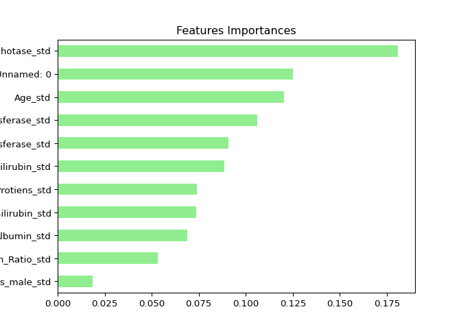
Apparently, hr and workingday are the most
important features according to rf. The importances of
these two features add up to more than 90%!